Interactive Ising Model in the Browser


Introduction to the Ising Model

The Ising model is a mathematical model used in statistical physics to study ferromagnetic materials such as iron. It consists of a large lattice of \( N \) sites, where the \( i^{th} \) site can be in either one of two states: \( \sigma_{i} = +1 \) (spin-up) or \( \sigma_{i} = -1 \) (spin-down). This project uses a square lattice, as shown in figure 1.

Any particular spin on the lattice feels the influence of its nearest-neighbouring spins, as measured by an interaction term, \( J_{ij} \). When \( J_{ij} > 0 \), neighbouring spins prefer to align with one another to minimise the energy of the system. Conversely, when \( J_{ij} < 0 \), neighbouring spins tend to anti-align into a checker-board-type pattern. Spins with \( J_{ij} = 0 \) are non-interacting. Figure 2 shows the interactions of a spin with its 4 nearest-neighbours on a square lattice.

Finally, the lattice can be subject to an external magnetic field, the strength of which is represented by \( h_{j} \) at site \( j \).

With these parameters, the Hamiltonian (total energy) of the system can then be written as: \[ H(\sigma) = -\sum\limits_{\langle ij \rangle} J_{ij} \sigma_{i} \sigma_{j} - \sum\limits_{j} h_{j} \sigma_{j}, \] where the angle brackets, \( \langle ij \rangle \) denote a sum over nearest-neighbours. In this particular project, however, we will not apply an external magnetic and the interaction strength will be constant, which simplifies the Hamiltonian to: \[ H(\sigma) = -J \sum\limits_{\langle ij \rangle} \sigma_{i} \sigma_{j}. \] In the Monte Carlo simulation method detailed in the next section, it is convenient to express the Hamiltonian in terms of a dimensionless interaction parameter, \( \epsilon = k_{B}T/J \), where \( k_{B} \) is Boltzmann's constant and \( T \) is temperature, leaving us with: \[ \frac{H(\sigma)}{k_{B}T} = - \frac{1}{\epsilon} \sum\limits_{\langle ij \rangle} \sigma_{i} \sigma_{j}. \]
Figure 1 - A 6x6 square Ising lattice representing a ferromagnet. Spins can be up (+1) or down (-1).
Figure 2 - Diagram showing the interactions (green) of a spin with its 4 nearest-neighbours.

Monte Carlo Simulation Method

In statistical physics, a system with fixed volume and number of particles in contact with a heat bath at a fixed temperature is referred to as a canonical ensemble. The partition function for a canonical ensemble, such as our Ising model, is given by \[ Z = \sum\limits_{i} e^{- \beta E_{i}}, \] where \( E_{i} \) is the energy of microstate (specific configuration) \( i \) and \( \beta = 1/k_{B}T \). Using the partition function, it is possible to calculate the thermodynamic average of a system observable, \( A \), via: \[ \langle A \rangle = \frac{1}{Z} \sum\limits_{i} A_{i} e^{- \beta E_{i}}, \] where \( A_{i} \) is the value of observable \( A \) in state \( i \). For example, the thermodynamic average of the energy would be: \[ \langle E \rangle = \frac{1}{Z} \sum\limits_{i} E_{i} e^{- \beta E_{i}}. \] The problem is that the number of states in a system becomes so large that we can't possibly count them and calculate the partition function directly. This is where Monte Carlo simulations come in...

Monte Carlo simulations create what is known as a 'Markov chain', where the next state to be visited depends only on the current state. The parition function of the system is effectively sampled by visiting each system-state with the correct probability - less-likely states are visited fewer times that likely states. Samples of observables (such as energy) are taken periodically as the system evolves and subsequently averaged. The longer the simulations runs for (more states visited), the more accurately the Monte Carlo averages will approximate the true thermodynamic values. The algorithm used to update the system in this project is summarised as follows:

Monte Carlo Metropolis algorithm:


  1. Randomly pick a lattice site, \( s \), from the lattice.
  2. Calculate the energy, \( E_{i} \), arising from the spin at site \( s \) interacting with its nearest-neighbours.
  3. Flip the spin at site \( s \) and calculate the energy of interaction, \( E_{j} \), arising from this new state.
  4. Calculate \( \Delta E = E_{j} - E_{i} \), the change in energy in moving from state \( i \) to state \( j \).
  5. Accept the new state, \( j \), with probability \( P_{i \rightarrow j} = \min(1, \exp(-\Delta E/k_{B}T)) \). Otherwise, put the system back in state \( i \).
  6. Sample any system observables and move back to step 1.

Note that since flipping a spin is a local move (i.e., the rest of the system remains unchanged), we don't have to recalculate the energy of the entire system, which save a lot of computation time.

Project Motivation

Existing Ising models on the web (to my knowledge):


  1. Single temperature.
  2. Single lattice size.
  3. Don't show how thermodynamic quantities vary with temperature (the interesting stuff in statistical physics!).
  4. Don't show the effect of finite-size effects (bigger systems give more realistic results).
  5. Speed often limited by screen refresh rate if animated, since calculations run on the main thread.
  6. Not usually any output graphs.

Benefits of this project:


  1. An 'experiment' corresponds to a particular size of Ising lattice.
  2. In each 'experiment', multiple Ising models are run at different temperatures simultaneously. E.g., a (20x20) Ising model with \( k_{B}T/J = 2.1,2.2,2.3,2.4 \).
  3. Multiple 'experiments' can be run simultanously. E.g., ten (20x20) Ising models in experiment #1 and eight (40x40) Ising models in experiment #2 running concurrently.
  4. Plots of magnetisation, energy, heat capacity, magnetic susceptibility and Binder fourth-order cumulant vs temperature.
  5. Results from the multiple temperatures in each 'experiment' are plotted in real-time as the simulations progress.
  6. The real-time data plots allow the user to see thermodynamic averages improving.
  7. Plotting multiple 'experiments' on a graph shows effects of the finite-size lattice on the results.
  8. The plot of Binder fourth-order cumulant allows the transition temperature to be detected regardless of finite-size effects.
  9. Results from each experiment are also shown in a data grid.
  10. Calculations run outside of the main thread.
  11. The configuration of any individual simulation can be shown in a pop-out window and is updated in real-time.
  12. The user can download the simulation data as a tab-delimited text file for further processing.

Instructions

Parameters Section


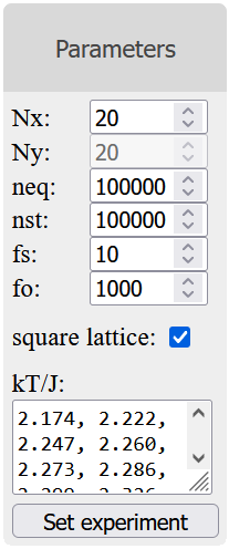
The parameters section, as shown in figures 3 and 4, allows the user to set up experiments. 
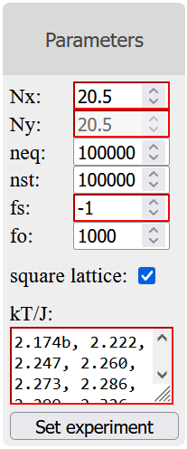
Any invalid parameters that have been entered will be highlighted in red. A new experiment cannot be set up until these fields have been corrected.

Param. Type Description
Nx Int (+) # lattice sites in x
Ny Int (+) # lattice sites in y
neq Int (+) # equilibration steps
nst Int (+) # statistics steps
fs Int (+) sample frequency
fo Int (+) output frequency
KT/J Float temperatures
Table 1 - Input parameters.

Table 1 briefly describes the input parameters. Quantities: \( n_{eq} \), \( n_{st} \), \( f_{s} \) and \( f_{o} \) are measured in units of "Monte Carlo steps per lattice site". I.e., setting \( n_{eq} = m \) results in \( m \times N_{x} \times N_{y} \) total Monte Carlo steps. This ensures that on average, each spin gets flipped the same number of times regardless of lattice size.

The simulations start by performing an equilibration period of length \( n_{eq} \). This gives the systems time to reach thermal equilibrium and no statistics are collected during this period.

A statistics period of length \( n_{st} \) follows the equilibration period, during which samples of the systems' thermodynamic variables are taken every \( f_{s} \) steps. Setting \( f_{s} \) too low causes subsequent samples to be highly correlated, which is detrimental to the averages. Setting it too high makes the averages take a long time to converge and appear noisy.

The output frequency, \( f_{o} \), sets how often the results are sent to the screen from the various simulations. Setting this number too low can make the chart animations appear jerky and, in the extreme, cause the configuration animations to start buffering .

Once valid parameters have been entered, clicking the "Set experiment" button will place a new experiment in the experiments section. Multiple experiments can be set up at the same time, as shown in figures 5 and 6. At this point, no simulations are running, they are simply in a state where they are waiting to be run.

Figure 3 - Input parameter fields.
Figure 4 - Invalid parameters.


Experiments Section


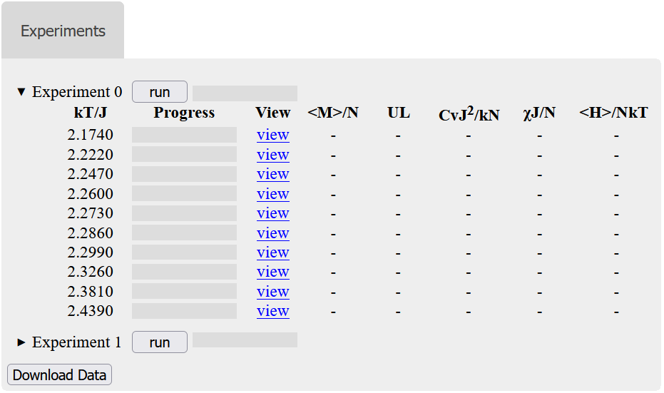
An experiment can be expanded by cliking on it to reveal a data grid, which is initially empty as in figure 5. Each row in the data frame corresponds to an Ising model simulation, but note that the view links will not work until the experiment is running.

Figure 5 - The experiments section displaying two experiments that are waiting to be run. Experiment 0 has its data grid expanded.
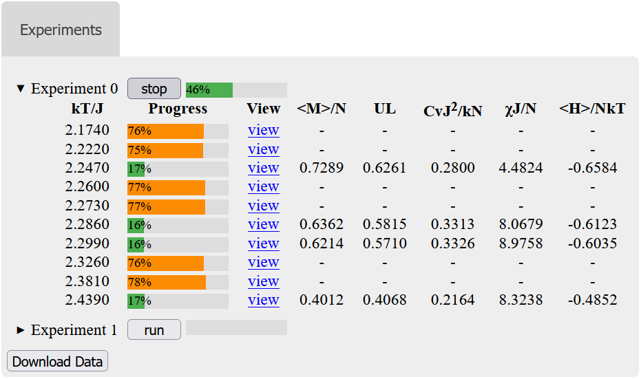
Figure 6 - The experiments section showing experiment 0 running with its data grid expanded. Experiment 1 is still waiting to be run.
Clicking on an experiment's 'run' button will start each of its consituent simulations. Figure 6 shows a running experiment where some experiments are in the equilibration phase (orange progress bar) and some have entered the statistics phase (green progress bar). The progress bar next to the 'run' button gives the total progress of the experiment as a whole. Simulations that are in the statistics phase have their row of the data grid updated every \( f_{o} \) steps.

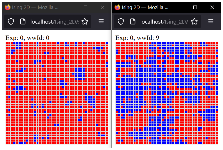
Once the experiment has started, clicking on one of the 'view' links will open a new window showing the current state of the configuration, as shown in figure 7. If the experiment is running, the configuration animation will be updated every \( f_{o} \) steps.

Clicking the 'Download Data' button allows the user to download all simulation data up to that point as a tab-delimited text file.

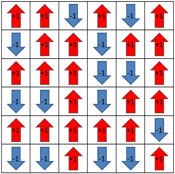
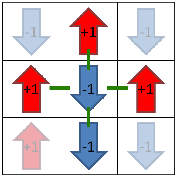
Figure 7 - Two (40x40) Ising model configurations at different temperatures, generated by clicking the 'view' links seen in figures 5 and 6.


Charts Section


Clicking the checkboxes in the 'charts' section shows/hides plots related to the various quantities detailed in table 2.

Chart Description
\( \langle M \rangle / N \) Magnetisation (scaled)
\( U_{L} \) 4th-order cumulant
\( C_{v}/(k_{B}N) \) Heat capacity (scaled)
\( \chi J / N \) Susceptibility (scaled)
\( \langle H \rangle / (Nk_{B}T) \) Energy (scaled)
Table 2 - Quantities plotted on charts.

The charts display the results from the experiments that the user has started. Each of the multiple data-series corresponds to a different experiment, which are updated every \(f_{o}\) steps throughout the simulation until it ends. 
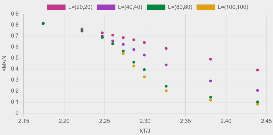
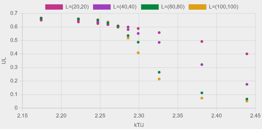
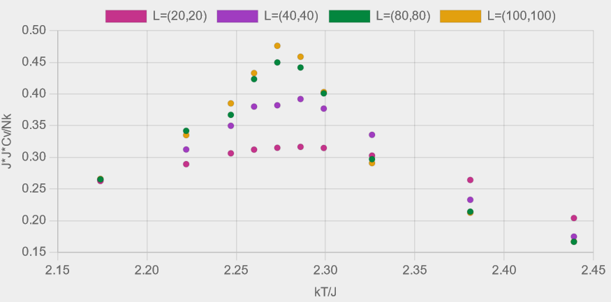
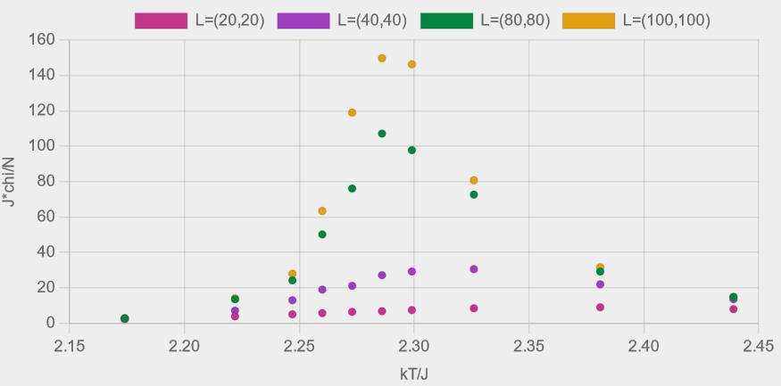
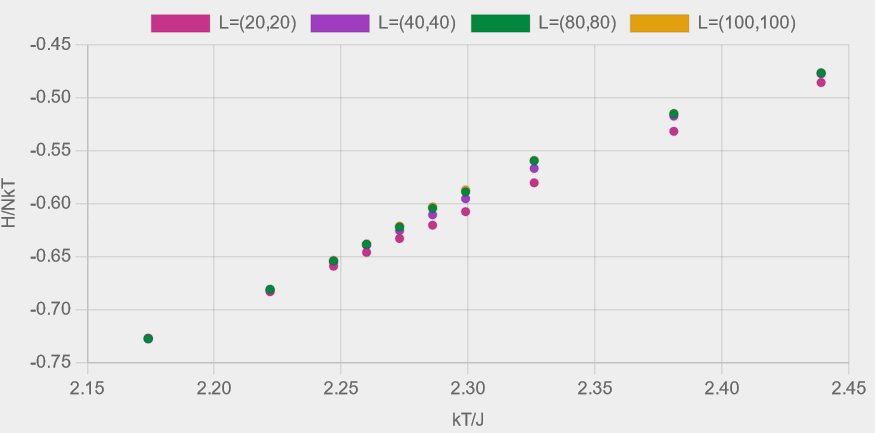
By displaying the results from experiments run at different lattice sizes, \( L=(N_{x}, N_{y}) \), on a single chart, the user is able to see both the quantity's temperature dependence and the effect of the finite-lattice size on the results.

Figures 8 (a)-(e) show the results from experiments with four different lattice sizes, \( L=(20,20), (40,40), (80,80) \) and \( (100,100) \), each comprising ten Ising model simulations run at temperatures spanning the critical temperature. The change in magnetisation across the transition clearly becomes steeper as lattice size increases towards an infinite system. As well as the peaks in the heat capacity and suceptibility becoming taller and narrower, the temperature at which the peaks occur also shift closer to the critical temperature.
Figure 8 - Plots of (a) magnetisation, (b) Binder fourth-order cumulant, (c) heat capacity, (d) susceptibility and (e) energy, as described in table 2. Each coloured dataset corresponds to a lattice of size \( L = (N_{x}, N_{y}) \).


Project Code


The (mostly javascript) code for this project can be seen on my github page at: https://github.com/tmbeardsley/ising2d_parallel/


Set up an experiment by adjusting the parameters...