Monte Carlo Simulations of Diblock Copolymers with an Interactive Front-End


Background Science


Diblock Copolymers (DBCs)


A diblock copolymer consists of an A-block of \( N_{A} \) segments and a B-block of \( N_{B} \) segments (figure 1), joined together at one end to give a linear chain with \( N = N_{A} + N_{B} \) total segments and composition fraction \( f_{A} = N_{A}/N \).


Figure 1 - A diblock copolymer with \( N_{A} \) segments in the A-block and \( N_{B} \) segments in the B-block.


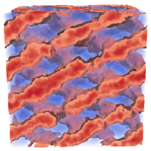
The strength of interactions between A and B segments is controlled by the Flory-Huggins parameter, \( \chi \), which is inversely related to temperature (i.e., low \( \chi \) corresponds to high temperature). When the A-B interactions in a melt of DBCs become sufficiently unfavourable (i.e., \( \chi \) becomes large enough) they microphase-separate, forming periodically ordered structures with domains on the nanometer scale. The equilibrium structures include the classical lamellar (L), cylindrical (C) and spherical (S) phases, as well as the complex gyroid (G) and Fddd phases (see figure 2).


Lamellar (L)
Cylinder(C)
Spherical (S)
Gyroid (G)
Fddd (Fddd)


Self-consistent Field Theory (SCFT)


Imagine looking at a single DBC in a melt. It has complicated interactions with all the other polymers in the system and capturing them all is a difficult mathematical and computational challenge. SCFT addresses this problem by replacing the interactions that a polymer has with other chains by mean fields.

Monodisperse Phase Diagram
SCFT has been enormously successful in the study of DBCs, producing the famous equilibrium phase diagram for a monodisperse melt shown in figure 3. It displays the various ordered phases, which are separated from the disordered phase by the order-disorder transition (ODT). It is also worth noting that the phase diagram is symmetric about \( f_{A} = 1/2 \).

Figure 3 - The self-consistent field theory phase diagram for diblock copolymer melts.
Figure 4 - A schematic representation of the effect of fluctuations on the SCFT phase diagram in figure 3.


Limitations of SCFT


Unfortunately, the mean-field nature of SCFT means that it doesn't include the fluctuation effects that are inherent in real statistical systems. As a result, we are interested in fluctuation corrections to figure 3, which are controlled by the invariant polymerisation index, \( \bar{N} = a^{6}\rho_{0}^{2}N \), where \( \rho_{0} \) is the segment density and \( a \) is the statistical segment length.

SCFT corresponds to the case where \( \bar{N} = \infty \), with fluctuations increasing as \( \bar{N} \) is reduced. The main effects of fluctuations on the monodisperse phase diagram in figure 3 are that the ODT gets shifted upward, and we get direct transitions between the disordered and ordered phases. For example, there will be a direct transition beween gyroid and disorder as indicated schematically in figure 4.

Monodisperse Phase Diagram from Experiments


In 1994, Bates et. al. performed experiments to produce monodisperse phase diagrams for three different DBC chemistries: PE-PEP (\( \bar{N}=27 \times 10^{3} \)), PEP-PEE (\( \bar{N}=3.4 \times 10^{3} \)) and PI-PS (\( \bar{N}=1.1 \times 10^{3} \)). Each of the phase diagrams exhibited the spherical, cylindrical and lamellar phases, but no gyroid or Fddd. There was, however, a region of another phase known as perforated lamellar in the region where SCFT predicts gyroid. Indeed, later experiments by Hajduk et. al. and Vigild et. al. showed that perforated lamellar is actually a long-lived metastable state that eventually converts to gyroid. Even more recent experiments by Wang et. al. and Takenaka et. al. have also confirmed the presence of Fddd on both sides of the phase diagram.

Whilst the experiments and SCFT phase diagrams exhibit a lot of good qualitative agreement, the significant differences are due to the effects of fluctuations near the ODT in the experiments: the shifting up of the ODT and direct transitions between disorder and the ordered phases.


Project Motivation


Scientific Motivation


  1. Use Monte Carlo simulations (more details in a previous project) to investigate the effects of fluctuations on diblock copolymer melts.
  2. Provide a real-time, visual output for the underlying Monte Carlo model to facilitate quick inspection of the system configuration/properties and aid parameter tuning.

Technical Motivation


  1. The fast inspection of system configurations and properties aids in quickly tuning parameters that can then be used in faster simulations (no front-end) for longer runs.
  2. Thermodynamic averages/statistics can be collected and displayed in charts in real-time as the simulation progresses (quicker than having to plot data files from a command-line program).

Simulation Code Requirements


Broad Simulation Requirements


  1. Create a visual front-end that allows the user to specify input parameters and displays the system configuration/data in real-time.
  2. Define a 3D lattice and generate an intial configuration.
  3. Use a Monte Carlo model (treats fluctuation effects) as the underlying engine on the back-end.
  4. Display performance-related information, such as time taken per Monte Carlo update and simulation progress.
  5. Display quantities such as the structure function, \( S(k) \) and energy, \( U \).
  6. Allow the user to control how often the configuration display is updated (frequent updates will limit simulation speed).

Technical Simulation Requirements


  1. Employ the lattice Monte Carlo model detailed previously (but without parallel tempering) for the back end.
  2. Use C# language as it is easy to build an interactive front-end with Windows Presentation Foundation (WPF).
  3. Port the Monte Carlo code from C/C++ to C# (relatively simple due to the similarity of the languages).
  4. Run the Monte Carlo simulation on background worker threads to keep the front-end responsive.
  5. Use the Helix Toolkit library (allows rotation and zooming) to display the system configuration.

Monte Carlo Methods (briefly)

In statistical physics, a system with fixed volume and number of particles in contact with a heat bath at a fixed temperature is referred to as a canonical ensemble. The partition function for a canonical ensemble, such as our diblock copolymer melt, is given by \[ Z = \sum\limits_{i} e^{- \beta E_{i}}, \] where \( E_{i} \) is the energy of microstate (specific configuration) \( i \) and \( \beta = 1/k_{B}T \). Using the partition function, it is possible to calculate the thermodynamic average of a system observable, \( A \), via: \[ \langle A \rangle = \frac{1}{Z} \sum\limits_{i} A_{i} e^{- \beta E_{i}}, \] where \( A_{i} \) is the value of observable \( A \) in state \( i \). For example, the thermodynamic average of the energy would be: \[ \langle E \rangle = \frac{1}{Z} \sum\limits_{i} E_{i} e^{- \beta E_{i}}. \] The problem is that the number of states in a system becomes so large that we can't possibly count them and calculate the partition function directly. This is where Monte Carlo simulations come in...

Monte Carlo simulations create what is known as a 'Markov chain', where the next state to be visited depends only on the current state. The parition function of the system is effectively sampled by visiting each system-state with the correct probability - less-likely states are visited fewer times that likely states. Samples of observables (such as energy) are taken periodically as the system evolves and subsequently averaged. The longer the simulations runs for (more states visited), the more accurately the Monte Carlo averages will approximate the true thermodynamic values. The algorithm used to update the system in this project is summarised as follows:

Monte Carlo Metropolis Algorithm


  1. The system begins in a state, \( i \), with energy \( U_{i} \).
  2. By performing one of the prescribed Monte Carlo moves, a small perturbation is made to the initial configuration in an attempt to move the system to state \( j \), with energy \( U_{j} \).
  3. The difference in energy, \( \Delta U = U_{j} - U{i} \), that would result from moving the system from state \( i \rightarrow j \) is calculated.
  4. If \( \Delta U \leq 0 \), then the accepted move from state \( i \rightarrow j \) is accepted, the system configuration is updated and we move to step 6.
  5. If \( \Delta U > 0 \), the system is attempting to adopt a higher energy state. In this case, generate a random number, \( R \). If \( R < \exp(-\Delta U / k_{B}T) \) then the move from \( i \rightarrow j \) is accepted and the system configuration updated. Otherwise, the system remains in the initial state, \( i \).
  6. Take samples contributing to Monte Carlo averages.
  7. Go to step 1 and repeat.

Benefits of Monte Carlo


There are many benefits to using the Monte Carlo method in this project, but the particularly significant ones are as follows:

Fluctuations are included
Because the Monte Carlo algorithm samples from the entire partition function of the system, this method inherently includes the effects of thermal fluctuations. This is in contrast to SCFT where the polymer interactions are approximated by mean-fields, thereby ignoring the fluctuation effects that are likely responsible for the differences between the theory and experiments (see section: 'Background Science').

Unphysical moves are permitted
The Monte Carlo algorithm is concerned with equilibrium behaviour and not the dynamics of how it gets from one state to another. It simply needs to sample all of the system's configurational states with the correct probabilities.

The desired property of the algorithm being able to reach every possible state is referred to as 'ergodicity'. The configuration space should be sampled as broadly and as quickly as possible, since it would be detrimental to our Monte Carlo averages to get stuck in a non-equilibrium state or to be cycling between only a few states. We attempt to make the system ergodic by a wise choice of Monte Carlo moves/updates, which do not have to obey physics in moving the system from state \( i \rightarrow j \). They can be anything we can think of that gets us to another valid state of the system. The snake, crank and flip moves used in this project are described in the section, 'Lattice Monte Carlo Simulation Details'.

Lattice Monte Carlo Simulation Details


Lattice Model Description


Each molecule in the system has \(N_{A}\) A-type monomers and \(N_{B}\) B-type molecules, such that there are \( N = N_{A} + N_{B} \) in total in a particular diblock. The monomers are placed on a lattice such that each lattice site may be vacant or occupied by a single monomer and bonded monomers must occupy nearest-neighbour sites. Although it would be more physically realistic to perform the simulations in free-space, a lattice construction is far less computationally expensive and allows for more Monte Carlo statistics to be collected per unit time.

The lattice is contructed by starting with an \( L \times L \times L \) cubic lattice with \( V_{c} = L^{3} \) sites and lattice constant, \( d \). The allowed lattice vectors can be described by \( {\bf r}_{i} = d(h,k,l) \), where \( i = 1,2,\ldots,L^{3} \) is the site number and \( h,k,l = 0,1,\ldots,L-1 \). By allowing only sites where \( h+k+l \) is even, a face-centred cubic (fcc) lattice with bond length \( b = \sqrt{2} d \) and \( V = V_{c}/2 = L^{3}/2 \) sites results. An fcc construction is used as its large coordination number (number of nearest-neighbours a particular site has) of \( z = 12 \) helps to alleviate the effects of the lattice. Periodic boundary conditions are implemented in all three dimensions to reduce the effects of the finite lattice size, requiring that \(L\) is an even number. The periodic boundary conditions mean that a molecule can travel off a face of the lattice and continue on the opposite face.

To allow the molecules room to move around and for the Monte Carlo algorithm to become efficient, the lattice is filled to a copolymer concentration of \( \phi_{c} \equiv nN/V \approx 0.8 \), where n is the total number of molecules in the system. Ideally, all lattice sites would be occupied, but this would make the Monte Carlo algorithm more complex, reducing its speed and the size of the systems that could be investigated.

Molecular interactions within the system occur only between nearest-neighbour A and B monomers. The strength of the interaction is given by \( \epsilon_{AB} \), from which a dimensionless Flory-Huggins parameter \[ \chi \equiv \frac{z\epsilon_{AB}}{k_{B}T} \] is defined.

At each Monte Carlo step (MCS), an attempt is made to change the system slightly by performing one of the available local moves. If the attempted move results in double occupancy of any lattice site, it is immediately rejected according to the Metropolis algorithm described in section 'Monte Carlo Methods'.

Local Monte Carlo Moves


Selection and implementation of the allowed Monte Carlo moves can have a large effect of the efficiency of the Monte Carlo algorithm. The moves should quickly update the system's configuration and efficiently sample its phase space. At each MCS, one of three moves: snake, crank or flip (figs 7a-c), is randomly attempted according to the predefined probabilities: \( P_{snake} = 0.45 \), \( P_{crank} = 0.45 \) and \( P_{flip} = 0.10 \).

Figure 5a - Snake move. The molecule attempts to move into a randomly picked site at its head or tail.
Figure 5b - Crank move. One of the non-end monomers attempts to move to a neighbouring site without changing its two bonded monomers.
Figure 5c - Flip move. The positions of monomers \( i \) and \( N-i \) are exchanged for the integers, \( s = 1 \) to \( N \).


Snake move
One of the system's \( 2n \) polymer-end monomers is randomly chosen, as well as one of its 12 nearest-neighbour sites. An attempt is made to move the chosen end-monomer into the selected site by shifting all the monomers comprising the molecule along the chain backbone, as in figure 7a. If the neighbouring site is occupied then the move is rejected, unless it's occupied by the monomer of the opposite chain end. In this case, all of the monomers shift around the loop without any double occupation occurring. The computational cost of the snake move is relatively low because the resulting energy change is calculated from only the contacts of the molecule's end and junction monomers.

Crank move
One of the system's \( n(N-2) \) non-end monomers is randomly chosen. An attempt is made to move the selected monomer into a neighbouring site while leaving the two monomers it is bonded to unchanged, as in figure 7b. Due to the fixed bond length, \( b \), required by the fcc lattice geometry, the possible bond angles and number of potential moves available to the selected monomer are \( 180^{\circ} \) (0), \( 120^{\circ} \) (1), \( 90^{\circ} \) (3) and \( 60^{\circ} \) (3). A \( 180^{\circ} \) bond angle leads to the move being immediately rejected since the monomer cannot be displaced. Otherwise, the number of neighbouring vacant sites that satisfy the bond angle are counted. If there are no vacant sites then the move is rejected. In all other cases, one of the vacant sites is chosen at random and the monomer is moved there. The crank move is computationally inexpensive since it only involves a single monomer.

Flip move
An attempt is made to flip a molecule randomly chosen from the system's \( n \) chains. This is achieved by swapping the positions of monomers \( i \) and (\( N-i \)) for all integers in \( i = 1 \) to \( N/2 \), as in figure 7c. Since the molecule already occupies the space it requires, it will never be rejected as a result of double site occupation. However, the flip move is computationally expensive compared the the snake and flip moves since the nearest neighbour contacts of each monomer in the chain must be counted.


Program User Guide


Setup and Input Parameters


After running the program, the first window presented to the user is shown in Figure 6. The "Input Parameters" section is populated with some initial values that can be edited by the user (the individual parameters are described in the next section).

Once finished editing the parameters, clicking the "Set up" button will validate that the parameters represent a valid simulation. If validation fails, the user is represented with an error message instructing them on how to fix the issue(s). After passing validation, the Monte Carlo back-end proceeds to generate an initial configuration as shown in Figure 7.

Figure 6 - The initial state of the program when it is first started. Clicking the "Set up" button validates the input parameters and generates an initial state.


Setup and Input Parameters


\( L \)
Number of sites along the \( x,y,z \) dimensions of the simulation box.

\( M \)
Total number of polymers in the system.

\( N \)
Total number of monomers in an \(AB\)-diblock copolymer.

\( N_{A} \)
Number of monomers in the \(A\)-block of an \(AB\)-diblock copolymer.

\( \chi N \)
The Flory-Huggins interaction parameter multipled by \( N \). Dictates the energy penalty of \(A-B\) monomer interactions.

\( n_{\textrm{relax}} \)
Length of relaxation period before sampling system statistics (in units of Monte Carlo steps per monomer).

\( n_{\textrm{estim}} \)
Length of statistics gathering period (in units of Monte Carlo steps per monomer).

\( f_{\textrm{sample}} \)
Period between taking samples in the estimation phase (in units of Monte Carlo steps per monomer).

\( (P_{\textrm{snake}}, P_{\textrm{flip}}, P_{\textrm{crank}}) \)
Cumulative probabilities with which the snake, flip and crank moves are attempted (must sum to one). E.g., \( (0.45, 0.55, 1.0) \) attempts the snake move 45% of the time, the flip move 10% of the time and the crank move the remaining 45% of the time.


Initial Configuration and Interacting with the Viewer


Once the input parameters have been validated, the Monte Carlo model sets up an initial configuration that is subsequntly displayed in the configuration viewer by the front-end (Figure 7). The user is then able to interact with the configuration:

Rotation:
Right-click and hold on the configuration. Moving the mouse then allows the configuration to be rotated in any direction.

Zoom:
Scroll the mouse wheel on the configuration to zoom in/out.

Translate:
Push and hold the middle mouse button on the configuration. Moving the mouse then allows the configuration to be translated within the viewer.

Reset View:
Double clicking the middle mouse button in the configuration viewer will reset the view to its default position.


Figure 7 - The state of the program after the "Set up" button has been clicked and the input parameters have been validated. An initial state has been generated and is displayed in the configuration viewer (can be zoomed and rotated). Subsequently clicking the "Run" button will start the Monte Carlo simulation.


Running the Simulation and Viewing its Status


After inspecting the initial (non-equilibrium) configuration, the user can click the "Run" button to start the Monte Carlo simulation. The simulation's progress is displayed to the user in the "Status" Section, as shown in Figure 8 and decribed below:

Equilibration:
The percentage of the simulation's equilibration (relaxation) period completed. Displayed as text and a progress bar.

Statistics:
The percentage of the simulation's statistics period completed. Displayed as text and a progress bar.

Sweep #:
The step number reached by the simulation at the last update of the front-end (in units of Monte Carlo steps per monomer).

ms/sweep:
The average amount of time (in milliseconds) for the system to attempt an update of every monomer in the system.


Figure 8 - The state of the program after the "Run" button has been clicked and the system is part way through a simulation. The "Controls" section allows the user to change parameters related to redrawing the configuration (less drawing leads to faster progress through the Monte Carlo simulation).


Using the Controls


While the simulation is running, the "Controls" section allows the user to alter how the configuration is displayed, as well as how often. The various controls are detailed as followed:

"Update Plot" Checkbox:
Switches on/off updates of the configuration display (the simulation continues in the background).

"AB-A-B" Radio Group:
Selects whether to display all monomers (AB), A-monomers (A) or B-monomers (B).

"Update Freq" Slider:
Specifies how often to update the configuration displayed on the front-end.

"Shell Depth" Slider:
The number of lattice layers (from the outside in) that are displayed when drawing the configuration.


Efficiency Considerations


It should be noted that displaying the configuration too often can negatively impact the speed of the Monte Carlo simulation. The size of the effect depends upon a number of factors, including simulation box size, but can be mitigated to a large extent by our choice of display control parameters:

  1. We are usually interested in observing the faces of the simulation box, which obscure the inside from view. Using the "Shell Depth" slider to display only one or two layers stops the internal (unobservable) layers from being drawn, saving computational effort and increasing simulation speed. If the internal layers need to be observed (e.g., checking domain purity while displaying only A or B monomers), the shell depth can be momentarily increased.

  2. Reducing how often the configuration is redrawn via the "Update Freq" slider will take fewer computational resources away from the Monte Carlo simulation working in the background. Alternatively, unticking the "Update Plot" checkbox will have the most drastic effect.

When altering the display parameters, the user should observe their effects on the "ms/sweep" in the "Status" section (a lower number is better).


Program Code


Coming soon -> This project is still a work in progress.

Although the core simulation and front-end are functioning correctly, there are a number of features that are not yet fully implemented, including real-time chart updates that will display the system's thermodynamic averages (concept already proven). As such, the program will be made available once these features have been added and tested.