Subsections
- Propagator Calculation
- Calculating \( \partial \ln (Q) / \partial L \) to determine equilibrium box size
- Random Number Generation
- Langevin update of \( W_{-}({\bf r}) \)
- Partition Function, \( Q \)
- Composition and Pressure fields, \( \phi_{-}({\bf r}) \) and \( \phi_{+}({\bf r}) \)
- Calculation of the Order Parameter, \( \Psi \)
Propagator Calculation
Without going into the full
mathematical details,
the simulation needs to calculate the composition field, \( \phi_{-}({\bf r}) \), and total concentration field, \( \phi_{+}({\bf r}) \)
multiple times in order to obtain \( w_{+} \) and update \( W_{-}({\bf r}) \) at each time step of the simulation.
However, \( \phi_{-}({\bf r}) \) and \( \phi_{+}({\bf r}) \) themselves necessitate calculation of forward and backward propagators given by the recursion relations:
\[ q_{i+1}({\bf r}) = h_{i+1}({\bf r}) \int g(R) q_{i}({\bf r} - {\bf R}) d{\bf R}, \]
\[ q_{i-1}^{\dagger}({\bf r}) = h_{i-1}({\bf r}) \int g(R) q_{i}^{\dagger}({\bf r} - {\bf R}) d{\bf R}, \]
where \( i \) indexes the polymer segment, \( h_{i}({\bf r}) \) is related to the \( i^{th} \) monomer's field energy and \( g({\bf r}) \) is
related to the stretching energy of polymer bonds (
mathematical details).
Calculating the propagators from these recursion relations is the most costly part of the FTS simulations,
which involves transforming to and from reciprocal space for \( N-1 \) of the monomers.
Since there are both forward and backward propagators, this results in \( 2(N-1) \) fast Fourier transforms (FFTs) having to be performed every time
\( \phi_{-}({\bf r}) \) and \( \phi_{+}({\bf r}) \) are calculated.
Then, considering the fact that \( \phi_{-}({\bf r}) \) and \( \phi_{+}({\bf r}) \) have to be recalculated \( n_{AM} \) times
at each time step of the simulation in order to solve the self-consistent equation for \( w_{+} \), the total number of
FFTs per time step, \( 2(N-1)n_{AM} \), soon adds up.
In serial versions of the code, the transforms are done with the
FFTW fast Fourier transform library.
However, performing Fourier transforms is highly parallelisable so this portion of the code has been rewritten to take advantage of the
CUDA
cuFFT library on the GPU.
In order to maximise the benefits of performing FFTs on the GPU, there are a number of other considerations that must be taken into account.
Minimising Data Transfers
Firstly, it is important to minimise the number of data transfers between CPU (host) memory and GPU (device) memory due to the costly
overhead associated with copying data between them.
As a result, the code has been written such that all of the propagators are calculated on the GPU without any need for any memory to be
copied to the host. This required that \( h_{i}({\bf r}) \) and \( g({\bf r}) \) were both calculated and accessible in GPU memory.
Batched FFTs
Secondly, performing an FFT using either the FFTW or cuFFT libraries requires setup of a "plan".
A plan provides the FFT library with the information it needs to perform the FFT, such as whether to do a forward/backward transform
and the size/dimensionality of the mesh. Two plans are required in this code: one for transforming from real to reciprocal space, the other for
transforming in the reverse direction.
Since we must calculate recursion relations for forward and backward propagators, a sensible first approach would be the following:
- Set up plans for forward (\( \mathcal{F_{r \rightarrow k}} \)) and backward (\( \mathcal{F_{k \rightarrow r}} \)) Fourier
transforms using the cufftPlan3d function of the cuFFT library.
- Set intial conditions, \( q_{i=1}({\bf r}) \) and \( q_{j=N}^{\dagger}({\bf r}) \), of the propagators.
- Calculate \( q_{i+1}({\bf r}) \), the forward propagator of monomer (\( i+1 \)), which involves transforms to and from reciprocal space
via the \( \mathcal{F_{r \rightarrow k}} \) and \( \mathcal{F_{k \rightarrow r}} \) cuFFT plans.
- Calculate \( q_{i-1}^{\dagger}({\bf r}) \), the backward propagator of monomer (\( j-1 \)), which involves transforms to and from reciprocal space
via the \( \mathcal{F_{r \rightarrow k}} \) and \( \mathcal{F_{k \rightarrow r}} \) cuFFT plans.
- Repeat steps 3-4 until \( q_{N}({\bf r}) \) and \( q_{1}^{\dagger}({\bf r}) \) have been calculated.
The above algorithm certainly works, but can be improved upon by considering that it may not be fully utilising the GPU.
To maximise throughput on the GPU (i.e., amount of calculations completed per unit time), we would ideally pass it
enough work that all its threads are utilised in parallel.
However, the FFTs being performed on the GPU in the algorithm above are limited by the simulation's 3D mesh size.
For example, suppose there are \( 60000 \) threads available on the GPU, but we run a simulation that uses only \( 30^{3} = 27000 \)
threads during a FFT. That means there are another \( 33000 \) threads not being used.
The problem is that in spite of having plenty of work for the GPU to do, we have to calculate the propagators sequentially since
\( q_{i+1}({\bf r}) \) depends on \( q_{i}({\bf r}) \) and \( q_{i-1}^{\dagger}({\bf r}) \) depends on \( q_{i}^{\dagger}({\bf r}) \) etc.
However, it should be noted that \( q({\bf r}) \) and \( q^{\dagger}({\bf r}) \) can be calculated independently of one another.
I.e., the calculations for \( q({\bf r}) \) do not have any dependence on \( q^{\dagger}({\bf r}) \) and vice versa.
Therefore, there would be no issue with calculating both of them at the same time if it were possible.
Fortunately, the cuFFT library provides us with the
cufftPlanMany()
function, which allows us to set up a plan where multiple Fourier transforms can be batch processed.
Put another way, cufftPlanMany() enables us to fast Fourier transform \( q({\bf r}) \) and \( q^{\dagger}({\bf r}) \) on the GPU at the same time,
thereby double the amount of required threads and taking better advantage of the hardware for smaller systems.
The only complication in batch processing \( q({\bf r}) \) and \( q^{\dagger}({\bf r}) \) is that they must be in contigious memory,
i.e., the arrays for \( q({\bf r}) \) and \( q^{\dagger}({\bf r}) \) must sit next to each other in the computer's memory.
As a result, the arrays in this simulation have been set up in such a way that \( q_{1}({\bf r}) \) and \( q^{\dagger}_{N}({\bf r}) \) reside next
to each other in memory, as do \( q_{2}({\bf r}) \) and \( q^{\dagger}_{N-1}({\bf r}) \) etc...
This reduces our algorithm to:
- Set up plans for forward (\( \mathcal{\hat{F}_{r \rightarrow k}} \)) and backward (\( \mathcal{\hat{F}_{k \rightarrow r}} \)) Fourier
transforms using the cufftPlanMany() function of the cuFFT library.
- Set intial conditions, \( q_{i=1}({\bf r}) \) and \( q_{j=N}^{\dagger}({\bf r}) \), of the propagators.
- Calculate \( q_{i+1}({\bf r}) \), the forward propagator of monomer (\( i+1 \)), and
\( q_{i-1}^{\dagger}({\bf r}) \), the backward propagator of monomer (\( j-1 \)),
at the same time via transforms to and from reciprocal space with the
(\( \mathcal{\hat{F}_{r \rightarrow k}} \)) and (\( \mathcal{\hat{F}_{k \rightarrow r}} \)) cufftPlanMany() plans
- Repeat step 3 until \( q_{N}({\bf r}) \) and \( q_{1}^{\dagger}({\bf r}) \) have been calculated.
Calculating \( \partial \ln (Q) / \partial L \) to determine equilibrium box size
For a cubic mesh, the equilibrium simulation box size can be determined by adjusting \( L_{\nu} \) until the ensemble averages of
\[ L_{\nu} \frac{\partial \ln (Q)}{\partial L} = \frac{L_{\nu}}{Q} \frac{\partial Q}{\partial L_{\nu}}, \]
are equal in each of the \( \nu = x,y,z \) dimensions. Here, \( L_{\nu} \) refers to the length of the box dimension and \( Q \) is the partition function.
In order to efficiently determine this quantity, propagators are calculated in reciprocal space.
While the mathematical details are not shown here
(see
Beardsley and Matsen, and
Riggleman and Fredrickson),
the calculation follows a very similar scheme to that detailed in the
Propagator Calculation section above.
As a result, all of the same GPU parallelisations are used in calculating \( \partial \ln (Q) / \partial L \) and the already allocated GPU memory can be reused.
There is also the benefit that this procedure also returns the partition function, \( Q \).
Random Number Generation
At each "time" step in the simulation, Gaussian random noise is added to the \( W_{-}({\bf r}) \) field at every point on the underlying mesh.
Since the total number of mesh point scales with the cube of the linear dimension
(i.e., a cubic mesh with linear dimension \( m_{x} = 64 \) has a total of \( M = m_{x}^{3} = 262,144 \) points),
there can be a significant number of random numbers and it makes sense to generate them in parallel on the GPU for speed.
Furthermore, having the random numbers already accessible on the GPU means that we can subsequently use them to update \( W_{-}({\bf r}) \)
on the GPU (see next section), rather than incurring the cost of copying the random numbers back to the CPU (host) and updating \( W_{-}({\bf r}) \) there.
To achieve GPU random number generation, I have taken advantage of the CUDA
cuRand library.
It has the advantage of the curandGenerateNormalDouble(...) function that generates normally distributed random numbers,
rather than having to generate a uniform random distribution and manually transform it:
curandGenerateNormalDouble(
curandGenerator_t generator,
double *outputPtr, size_t n,
double mean, double stddev
).
Langevin update of \( W_{-}({\bf r}) \) and \( W_{+}({\bf r}) \)
During testing, it was found that the Leimkuhler-Matthews algorithm previously used in
L-FTS
did not provide adequate stability in CL-FTS (the numerics would blow up within a relative short amount of simulation time).
Instead, a
predictor-corrector algorithm with adaptive time step was used (mathematics not detailed here).
The size of time step taken during each Langevin update is scaled with inverse proportion to the largest force being exerted on the fields.
This acts to make the simulation more stable by taking small time steps when forces are large, and larger time steps when the forces are small.
Fourtunately, this algorithm can be applied to each mesh point independently so the code has been written to update \( W_{-}({\bf r}) \) and \( W_{+}({\bf r}) \) in both
the predictor and corrector steps on the GPU. Furthermore, the function
thrust::max_element() uses the GPU
to rapidly identify the largest forcing term for implementing the adaptive time step.
Partition Function, \( Q \)
The partition function, \( Q \), is required for the Langevin update of \( W_{-}({\bf r}) \), as well in calculating
the composition field \( \phi_{-}({\bf r}) \), and the pressure field \( \phi_{+}({\bf r}) \). The simplest way to
calculate \( Q \) is to integrate the forward
propagator of the \( N^{th} \) monomer over all space:
\[ Q = \int q_{N}({\bf r}) d{\bf r}, \]
with the integral becoming a sum in the simulation code.
Since the propagator has already been computed on the GPU, it would be advantageous to calculate the sum there too, rather
than copy \( q_{N}({\bf r}) \) back to the CPU (host) for summation. Doing so requires a reduction
algorithm, so the
reduce(...) function of the
CUDA
Thrust library is used.
As a side note, \( Q \) is also calculated as a byproduct determining \( \partial \ln (Q) / \partial L \).
However, since the function to get \( \partial \ln (Q) / \partial L \) is not neccessarily called at each Langevin step,
the propagator reduction method (must be called at each step) remains the primary method of determining \( Q \).
Composition and Pressure fields, \( \phi_{-}({\bf r}) \) and \( \phi_{+}({\bf r}) \)
The composition and pressure fields form part of the update to \( W_{-}({\bf r}) \) and \( W_{+}({\bf r}) \) at the next time step.
These two fields are given by the equations
\[ \phi_{-}({\bf r}) = \frac{1}{NQ} \sum\limits_{i=1}^{N} \gamma_{i} \frac{q_{i}({\bf r}) q_{i}^{\dagger}({\bf r})}{ h_{i}({\bf r}) }, \]
and
\[ \phi_{+}({\bf r}) = \frac{1}{NQ} \sum\limits_{i=1}^{N} \frac{q_{i}({\bf r}) q_{i}^{\dagger}({\bf r})}{ h_{i}({\bf r}) }, \]
where \( \gamma_{i} = +1 \) if monomer \( i \) is A-type, or -1 if it's B-type.
These are costly fields to evaluate serially, because the product \( q_{i}({\bf r}) q_{i}^{\dagger}({\bf r}) \) has to be evaluated
\( N \) times for every mesh point.
However, as discussed in the previous sections, all of the quantities required in the above equations are already available on the GPU.
It is therefore straightforward to consider a single \( i \) and calculate \( q_{i}({\bf r}) q_{i}^{\dagger}({\bf r}) \) for all mesh points
in parallel.
By repeating this process for the \( i = 1 \ldots N \) monomers and summing the results, we vastly reduce the time taken to evaluate the fields.
Calculation of the Order Parameter, \( \Psi \)
As shown in detail in the
project applying metadynamics to L-FTS,
it was possible to identify the ordered phase via an order-parameter:
\[ \Psi = \frac{1}{R_{0}^{3}} \left( \frac{V}{(2 \pi)^{3}} \int f(k) \lvert W_{-}({\bf k}) \rvert^{l} d{\bf k} \right)^{1/l}, \]
where \( R_{0} \) is the end-to-end length of a polymer, \( V \) is the volume of the system and \( f(k) \) is a Heavide-like
screening function that limits the contribution of large wavevectors to the integral.
The parameter, \( l \), is chosen so that the \( \Psi \) exhibits a large value when the system is in the ordered phase and a small value in the disordered phase.
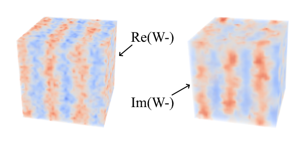
In L-FTS the fields are real-valued, so any choice of \( l \) will result in \( Psi \) being real-valued - this is not the case for the
complex fields in CL-FTS. Fortunately, the optimal choice of \( l=4 \) determined in L-FTS metadynamics reduces \( \Psi \) to:
\[ \Psi = \frac{1}{R_{0}^{3}} \left( \frac{V}{(2 \pi)^{3}} \int f(k) \lvert W_{-}({\bf k})W_{-}({\bf -k}) \rvert^{2} d{\bf k} \right)^{1/4}, \]
which continues to be real-valued in CL-FTS.
Calculating the order parameter requires a Fourier transform of the real-space field, \(W_{-}({\bf r}) \), into reciprocal space to obtain \( W_{-}({\bf k}) \).
A Fourier transform can be a costly operation to perform on the host (CPU), the execution time scaling with the number of mesh
points used to represent the field. It may also be the case that the user wishes to output \( \Psi \) at every
time step, so this relatively costly calculation could end up being performed frequently. As a result, I have used CUDA's CuFFT library
to perform the Fourier transform on the GPU with the function:
cufftResult
cufftExecD2Z(
cufftHandle plan,
cufftDoubleReal *idata,
cufftDoubleComplex *odata);
The next area that can be parallelised is identified by noting that the equation for the order parameter contains an integral
that becomes a summation on our discrete mesh:
$$\begin{equation}
\int f(k) \lvert W_{-}({\bf k}) \rvert^{l} d{\bf k} \rightarrow C \sum_{i} f(k_{i}) \lvert W_{-}({\bf k}_{i}) \rvert^{l}.
\end{equation}$$
If we look at the contribution to the sum from a particular wavevector \( {\bf k}_{i} \),
it's clear that neither \( f(k_{i}) \) or \( W_{-}({\bf k}_{i}) \) depend on any other wavevector, \( k_{j} \).
As a result, we can divide up the hard work by calculating each contribution in parallel on the GPU.
The next step would be to add the results from each \( k_{i} \) together again. We could achieve this by copying the
array of results from the GPU back to the host and summing them with the CPU. However, copying a large array between
host and GPU memory can become costly, especially if repeated often.
As a result, I have utilised the CUDA Thrust library function:
OutputType thrust::
transform_reduce(
InputIterator first,
InputIterator last,
UnaryFunction unary_op,
OutputType init,
BinaryFunction binary_op).
Whilst I will not go through the function in detail, it takes an iterator specifying the first and last positions of
the input arrays, a function that will be applied the the input data (in our case, it calculates the product
\( f(k_{i}) \lvert W_{-}({\bf k}_{i}) \rvert^{l} \)), the initial summation value (zero), and a reduction operator
(i.e., the built in operation
thrust::plus<double>()
for summation). These parameters are used to perform a sum of
the transformed input data on the GPU and finally return a single double precision variable (not a large array) to
host memory. In the code, the function looks like:
Psi = thrust::transform_reduce(
_z,
_z + _M,
Psi4_calc(),
0.0,
thrust::plus<double>());
where _z is a
thrust::zip_iterator<IteratorTuple>
(not discussed here), _M and _Mk are constants corresponding to array lengths in real and reciprocal space and the function:
Psi4_calc()
calculates the product \( f(k_{i}) \lvert W_{-}({\bf k}_{i}) W_{-}(-{\bf k}_{i}) \rvert^{2} \).
The steps outlined above are contained within the public function:
double get_Psi4(thrust::device_vector> &w_gpu, bool isWkInput = false)
in the order_parameter() class. It requires either a reference to \( W_{-}({\bf r}) \) (isWkInput = false),
or \( W_{-}({\bf r}) \) (isWkInput = true) stored on the GPU as a parameter.